2. Construction of expression matrix

2.1 Visualization: Genome Broswer

2.1.1 Build bedGraph/bigwig files

use BEDtools and UCSC Kent Utilities

# convert sam to bam
samtools view -S -b NC_1.miRNA_hg38_mapped.sam | samtools sort - > NC_1.miRNA_hg38_mapped.bam
# build bam index
samtools index NC_1.miRNA_hg38_mapped.bam > NC_1.miRNA_hg38_mapped.bai
# create bedGraph
bedtools genomecov -ibam NC_1.miRNA_hg38_mapped.bam -bga -split | sort -k1,1 -k2,2n > NC_1.miRNA_hg38_mapped.bedGraph

Note
http://bedtools.readthedocs.io/en/latest/content/tools/genomecov.html

use homer

1.Make tag directories for each experiment
```
#works with sam or bam (samtools must be installed for bam)
makeTagDirectory NC_1.miRNA.tagDir/ NC_1.miRNA_hg38_mapped.sam -format sam
```
If the experiment is strand specific paired end sequencing, add "-sspe" to the end. If it's unstranded paired-end sequencing, no extra options are needed.
makeTagDirectory tags_Dir/ inputfile.sam -format sam -sspe

2.Make bedGraph visualization files for each tag directory

# Add "-strand separate" for strand-specific sequencing
makeUCSCfile NC_1.miRNA.tagDir/ -fragLength given -o auto
(repeat for other tag directories)

2.1.2 Integrative Genomics Viewer(IGV)

https://igv.org/

in our case, try to load the bam and bigwig format file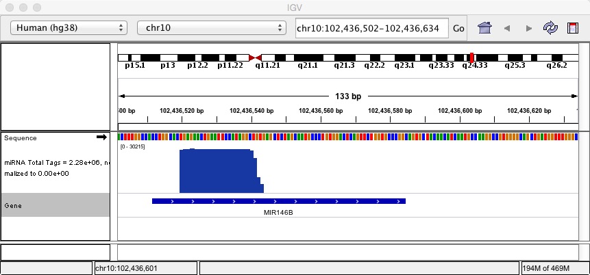

2.1.3 UCSC genome browser

https://genome.ucsc.edu/

2.2 Quantify gene expression

2.2.1 Concept

raw counts
RPKM: Reads Per Kilobase of exon model per Million mapped reads (每千个碱基的转录每百万映射读取的reads)
FPKM: Fragments Per Kilobase of exon model per Million mapped fragments(每千个碱基的转录每百万映射读取的fragments, 对于Pair-end sequencing, two paired reads should be mapped simultaneously)
```
RPKM = total exon reads/ (mapped reads (Millions) * exon length(KB))
```
TPM：Transcripts Per Kilobase of exon model per Million mapped reads (每千个碱基的转录每百万映射读取的Transcripts)
```
TPMi=(Ni/Li)*1000000/sum(Ni/Li+……..+ Nm/Lm)
```
RPM/CPM: Reads/Counts of exon model per Million mapped reads (每百万映射读取的reads)
```
RPM=total exon reads / mapped reads (Millions)
```

2.2.2 Required files

alignment: bam/sam format

convert sam to bam

samtools view -S -b NC1.miRNA_hg38_mapped.sam > NC1.miRNA_hg38_mapped.bam

annotaion: gtf/gff/gff3 format convert gff to gtf
```
gffread tRNA.gff -T -o tRNA.gtf
```

2.2.3 Tools

the gtf annotation should be match to the genome (index).
in our case, we build index for each RNA types, but the annotaion file (gff/gtf) is matched the position in human genome.

samtools view -bhF 4 NC1.miRNA.sam | bedtools bamtofastq -i - -fq NC1.miRNA_fastq
bowtie2 -p 4 --sensitive-local -x /BioII/lulab_b/shared/genomes/human_hg38/index/bowtie2_hg38_index/GRCh38_p10 NC1.miRNA_fastq -S NC1.miRNA_hg38_mapped.sam
samtools view -S -b NC1.miRNA_hg38_sam > NC1.miRNA_hg38_mapped.bam

* HTSeq

Given a file with aligned sequencing reads(.sam/.bam) and a list of genomic features(.gtf), a common task is to count how many reads map to each feature(gene).

Usage

htseq-count [options] <alignment_files> <gff_file>

in our case

htseq-count -m intersection-strict --idattr=Name --type=miRNA_primary_transcript NC_1.miRNA_hg38_mapped.sam /BioII/lulab_b/shared/genomes/human_hg38/gtf/miRNA.gff > NC_1.miRNA.htseq.counts

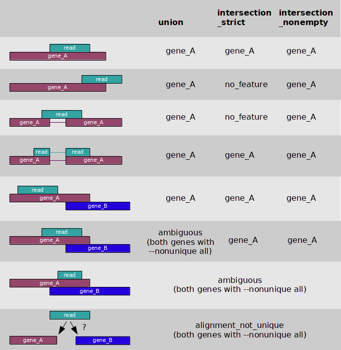
3 overlap resolution models
We shared our snakemake package used for exRNA-seq expression matrix construction.Github.

Tips

--nonunique
- --nonunique none (default): the read (or read pair) is counted as ambiguous and not counted for any features. Also, if the read (or read pair) aligns to more than one location in the reference, it is scored as alignment_not_unique.
- --nonunique all: the read (or read pair) is counted as ambiguous and is also counted in all features to which it was assigned. Also, if the read (or read pair) aligns to more than one location in the reference, it is scored as alignment_not_unique and also separately for each location.
- Notice that when using --nonunique all the sum of all counts will not be equal to the number of reads (or read pairs), because those with multiple alignments or overlaps get scored multiple times.

Notes

-m/--mode {mode}
--nonunique={none/all}
-s/--stranded {yes/no/reverse}.
-a {minaqual}.
-t/--type {feature type}. (defult: exon)
-i/--idattr {id attribute}, GFF attribute to be used as feature ID. (defult: gene_id)

* featureCounts

Usage

Summarize a BAM format dataset:

featureCounts -t exon -g gene_id -a annotation.gtf -o counts.txt mapping_results_SE.bam

Summarize multiple datasets at the same time:

featureCounts -t exon -g gene_id -a annotation.gtf -o counts.txt library1.bam library2.bam library3.bam

in our case

featureCounts -t miRNA_primary_transcript -g Name -a /BioII/lulab_b/shared/genomes/human_hg38/gtf/miRNA.gff -o NC_1.miRNA.featureCounts.counts NC_1.miRNA_hg38_mapped.bam

Tips
By default, featureCounts does not count reads overlapping with more than one feature. Users can use the -O option to instruct featureCounts to count such reads (they will be assigned to all their overlapping features or meta-features).

* Homer

Usage

0.Align FASTQ reads using STAR or similar 'splicing aware' genome alignment algorithm
1.Make tag directories for each experiment
```
#works with sam or bam (samtools must be installed for bam)
makeTagDirectory Exp1r1/ inputfile1r1.sam -format sam
makeTagDirectory Exp1r2/ inputfile1r2.sam -format sam
```
If the experiment is strand specific paired end sequencing, add "-sspe" to the end. If it's unstranded paired-end sequencing, no extra options are needed.
makeTagDirectory Exp1/ inputfile.sam -format sam -sspe

2. Quantify gene expression across all experiments for clustering and reporting (-rpkm):

# May also wish to use "-condenseGenes" if you don't want multiple isoforms per gene
analyzeRepeats.pl rna hg19 -strand both -count exons -d Exp1r1/ Exp1r2 Exp2r1/ Exp2r2/ -rpkm > rpkm.txt
# Use this result for gene expression clustering, PCA, etc.

3. Quantify gene expression as integer counts for differential expression (-noadj)

# May also wish to use "-condenseGenes" if you don't want multiple isoforms per gene
analyzeRepeats.pl rna hg19 -strand both -count exons -d Exp1r1/ Exp1r2 Exp2r1/ Exp2r2/ -noadj > raw.txt

in our case

makeTagDirectory NC_1.miRNA.tagDir/ NC_1.miRNA_hg38_mapped.sam -format sam
# raw counts
analyzeRepeats.pl /BioII/lulab_b/shared/genomes/human_hg38/gtf/miRNA.gtf hg38 -count exons -d NC_1.miRNA.tagDir/ -noadj > NC_1.miRNA.homer.counts
# calculate rpkm
analyzeRepeats.pl /BioII/lulab_b/shared/genomes/human_hg38/gtf/miRNA.gtf hg38 -count exons -d NC_1.miRNA.tagDir/ -rpkm > NC_1.miRNA.homer.rpkm
# calculate rpm/cpm
analyzeRepeats.pl /BioII/lulab_b/shared/genomes/human_hg38/gtf/miRNA.gtf hg38 -count exons -d NC_1.miRNA.tagDir/ -norm 1e7 > NC_1.miRNA.homer.rpm

Tips:
in default, homer do not use gff format file but gtf format.
look into the difference between:

/BioII/lulab_b/shared/genomes/human_hg38/gtf/miRNA.gtf
/BioII/lulab_b/shared/genomes/human_hg38/gtf/miRNA.gff

2.2.4 Merge to expression matrix

use linux command (cut, awk, sed, paste...)
generate expression matrix using homer:

analyzeRepeats.pl /BioII/lulab_b/shared/genomes/human_hg38/gtf/miRNA.gtf hg38 \
-d NC_1.miRNA.tagDir/ NC_2.miRNA.tagDir/ NC_1.miRNA.tagDir/ \
BeforeSurgery_1.miRNA.tagDir/ BeforeSurgery_2.miRNA.tagDir/ BeforeSurgery_2.miRNA.tagDir/ \
AfterSurgery_1.miRNA.tagDir/ AfterSurgery_2.miRNA.tagDir/ AfterSurgery_3.miRNA.tagDir/ \
-noadj > hcc_example.homer.ct.tsv

2.3 QC: Cleaning the expression matrix

* load expression matrix

# R script
> mx <- read.table("hcc_example.homer.ct.mx",sep="\t",header=T)
> head(mx[,1:5])
  TranscriptID NC_1 NC_2 NC_3 BeforeSurgery_1
1  hsa-mir-631    0    0    0               0
2 hsa-mir-4635    0    0    0               0
3 hsa-mir-6761    0    0    0               0
4  hsa-mir-10a 2533 1674 2744            3564
5 hsa-mir-2276    3    2    0               1
6 hsa-mir-4468    0    0    0               0

* check the library size

> colSums(mx[,2:ncol(mx)])
           NC_1            NC_2            NC_3 BeforeSurgery_1 BeforeSurgery_2
        2793900         2029386         3072213         6195915         4358534
BeforeSurgery_3  AfterSurgery_1  AfterSurgery_2  AfterSurgery_3
        3784022         3634594         6421256         2185529

* check total detected genes

> apply(mx[,2:ncol(mx)], 2, function(c)sum(c!=0))
           NC_1            NC_2            NC_3 BeforeSurgery_1 BeforeSurgery_2
            657             647             657             640             711
BeforeSurgery_3  AfterSurgery_1  AfterSurgery_2  AfterSurgery_3
            679             618             651             690

* filter genes

Purpose
Filtering low-expression genes improved DEG detection sensitivity.
Methods

Filter the genes with a total counts < = threshold;
Filter genes with maximum normalized counts across all samples < = threshold;
Filter genes with mean normalized counts across all samples < = threshold.

Criteria
Retain genes: (Reads >= 1 counts) >= 20% samples.

> filter_genes <- apply(
+    mx[,2:ncol(mx)], 
+    1, 
+    function(x) length(x[x > 2]) >= 2
+ )

> mx_filterGenes <- mx[filter_genes,]

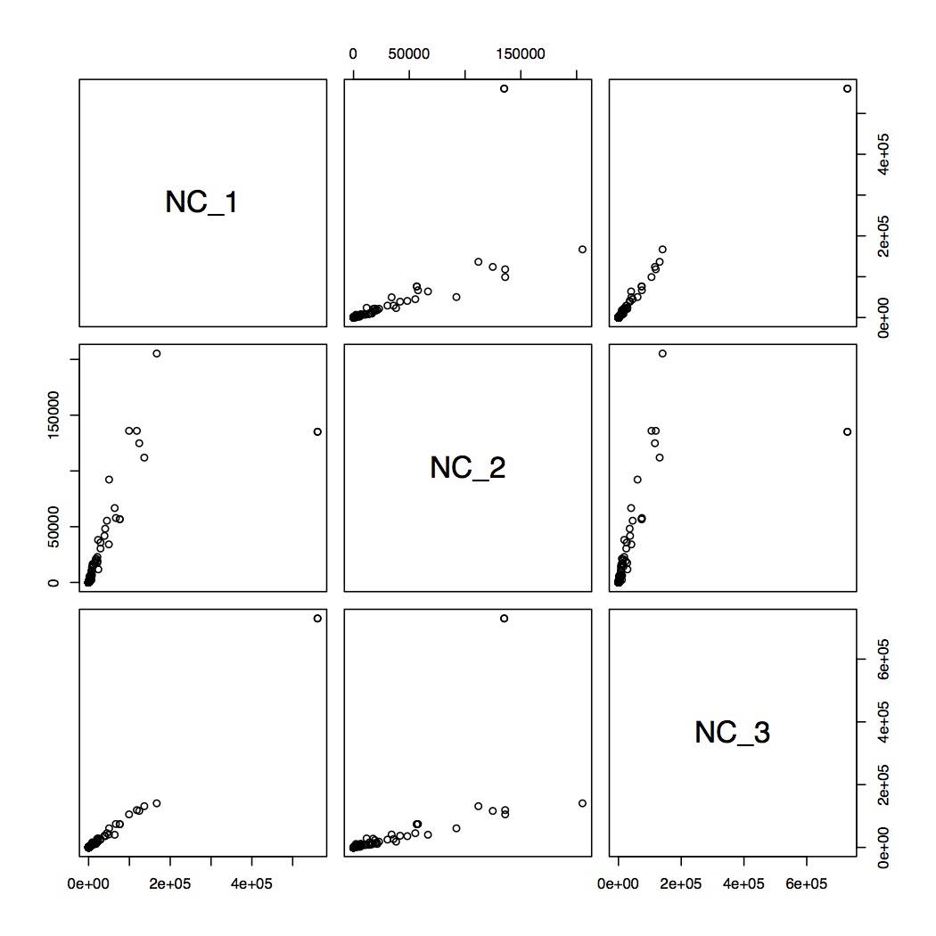
* check correlations between samples

> cor.test(mx_filterGenes$NC_1,mx_filterGenes$NC_2,methods="spearman")
> pairs(~NC_1+NC_2+NC_3,data=mx_filterGenes)
> dev.off()

Scripts summary

convert alignments

samtools view -bhF 4 NC1.miRNA.sam | bedtools bamtofastq -i - -fq NC1.miRNA_fastq
bowtie2 -p 4 --sensitive-local -x /BioII/lulab_b/shared/genomes/human_hg38/index/bowtie2_hg38_index/GRCh38_p10 NC1.miRNA_fastq -S NC1.miRNA_hg38_mapped.sam
samtools view -S -b NC1.miRNA_hg38_sam > NC1.miRNA_hg38_mapped.bam

count for expression value

# use htseq
htseq-count -m intersection-strict --idattr=Name --type=miRNA_primary_transcript NC_1.miRNA_hg38_mapped.sam /BioII/lulab_b/shared/genomes/human_hg38/gtf/miRNA.gff > NC_1.miRNA.htseq.counts
# use featureCounts
featureCounts -t miRNA_primary_transcript -g Name -a /BioII/lulab_b/shared/genomes/human_hg38/gtf/miRNA.gff -o NC_1.miRNA.featureCounts.counts NC_1.miRNA_hg38_mapped.bam
# use homer
analyzeRepeats.pl /BioII/lulab_b/shared/genomes/human_hg38/gtf/miRNA.gtf hg38 -count exons -d NC_1.miRNA.tagDir/ -noadj > NC_1.miRNA.homer.counts

generate expression matrix

# use homer
analyzeRepeats.pl /BioII/lulab_b/shared/genomes/human_hg38/gtf/miRNA.gtf hg38 \
-d NC_1.miRNA.tagDir/ NC_2.miRNA.tagDir/ NC_1.miRNA.tagDir/ \
BeforeSurgery_1.miRNA.tagDir/ BeforeSurgery_2.miRNA.tagDir/ BeforeSurgery_2.miRNA.tagDir/ \
AfterSurgery_1.miRNA.tagDir/ AfterSurgery_2.miRNA.tagDir/ AfterSurgery_3.miRNA.tagDir/ \
-noadj > hcc_example.homer.ct.tsv

cleaning the expression matrix

# R script
> mx <- read.table("hcc_example.homer.ct.mx",sep="\t",header=T)
> head(mx[,1:5])
  TranscriptID NC_1 NC_2 NC_3 BeforeSurgery_1
1  hsa-mir-631    0    0    0               0
2 hsa-mir-4635    0    0    0               0
3 hsa-mir-6761    0    0    0               0
4  hsa-mir-10a 2533 1674 2744            3564
5 hsa-mir-2276    3    2    0               1
6 hsa-mir-4468    0    0    0               0

# check library size (total mapped reads)
> colSums(mx[,2:ncol(mx)])
           NC_1            NC_2            NC_3 BeforeSurgery_1 BeforeSurgery_2
        2793900         2029386         3072213         6195915         4358534
BeforeSurgery_3  AfterSurgery_1  AfterSurgery_2  AfterSurgery_3
        3784022         3634594         6421256         2185529

# check the number of detected genes
> apply(mx[,2:ncol(mx)], 2, function(c)sum(c!=0))
           NC_1            NC_2            NC_3 BeforeSurgery_1 BeforeSurgery_2
            657             647             657             640             711
BeforeSurgery_3  AfterSurgery_1  AfterSurgery_2  AfterSurgery_3
            679             618             651             690

# filter genes
> filter_genes <- apply(
+    mx[,2:ncol(mx)], 
+    1, 
+    function(x) length(x[x > 2]) >= 2
+ )

> mx_filterGenes <- mx[filter_genes,]
> head(mx_filterGenes[,1:5])
   TranscriptID NC_1 NC_2 NC_3 BeforeSurgery_1
3  hsa-mir-6761    0    0    0               0
4   hsa-mir-10a 2533 1674 2744            3564
5  hsa-mir-2276    3    2    0               1
8   hsa-mir-100  540  165  516            2337
10 hsa-mir-371a    2    2    0               5
16 hsa-mir-3922    6    7    1               1

# check the correlations between each samples
> cor.test(mx_filterGenes$NC_1,mx_filterGenes$NC_2,methods="spearman")

    Pearson's product-moment correlation

data:  mx_filterGenes$NC_1 and mx_filterGenes$NC_2
t = 28.728, df = 616, p-value < 2.2e-16
alternative hypothesis: true correlation is not equal to 0
95 percent confidence interval:
 0.7208567 0.7885148
sample estimates:
      cor
0.7567047

> pairs(~NC_1+NC_2+NC_3,data=mx_filterGenes)
> dev.off()

# save the results
write.table(mx_filterGenes,"hcc_example.homer.ct.filtered.mx",sep="\t",quote=F,col.names=T,row.names=F)

Homeworks

scripts and files: /home/younglee/projects/bioinfoTraining/constructExpMx

Level I:

learn how to construct the expression matrix for gencode annotations and all RNA types (miRNA, piRNA, mRNA, lncRNA...)
compare the difference between HTSeq, featureCounts and homer
check the bam/bigWig file using IGV
QC and cleaning the expression matrix
Level II:
convert bam/sam files coordinates to genome coordinates

2.Construction of Expression Matrix

2. Construction of expression matrix

2.1 Visualization: Genome Broswer

2.1.1 Build bedGraph/bigwig files

use BEDtools and UCSC Kent Utilities

use homer

1.Make tag directories for each experiment

2.Make bedGraph visualization files for each tag directory

2.1.2 Integrative Genomics Viewer(IGV)

2.1.3 UCSC genome browser

2.2 Quantify gene expression

2.2.1 Concept

2.2.2 Required files

2.2.3 Tools

* HTSeq

* featureCounts

* Homer

0.Align FASTQ reads using STAR or similar 'splicing aware' genome alignment algorithm

1.Make tag directories for each experiment

2. Quantify gene expression across all experiments for clustering and reporting (-rpkm):

3. Quantify gene expression as integer counts for differential expression (-noadj)

2.2.4 Merge to expression matrix

2.3 QC: Cleaning the expression matrix

* load expression matrix

* check the library size

* check total detected genes

* filter genes

* check correlations between samples

Scripts summary

Homeworks

scripts and files: /home/younglee/projects/bioinfoTraining/constructExpMx

results matching ""

No results matching ""